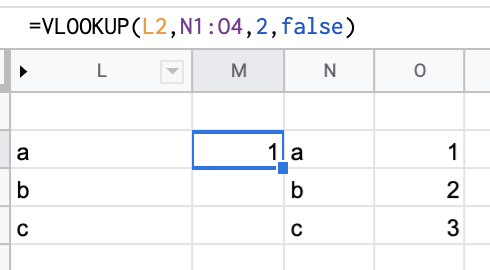
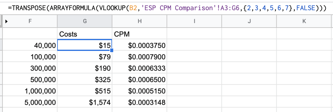
I know how to do a VLOOKUP in Google Sheets, but I didn’t know how to VLOOKUP the entire row. I solved this by nesting the VLOOKUP inside an ARRAY.
The quick solution for you to copy and paste is below, and the longer more detailed reasoning is at the bottom.
Here’s the Vlookup Formula
=ARRAYFORMULA(VLOOKUP(A1,'Sheet2'!A3:G6,{2,3,4,5,6,7},FALSE))
This takes the value in A1, searches for it in the array Sheet2!A3:G6, and returns the 2nd to 7th values in that row in order.
That formula will break if you add any columns, if that happens try this instead:
=ARRAYFORMULA(VLOOKUP(A1,'Sheet2'!A3:G6,COLUMN(B3:G6),FALSE))
Step-by-step Explanation
I’ve gotten to know Vlookups really well over the years. If you need a quick refresher, Vlookup is a great way to match data across columns or spreadsheets quickly. It takes a value in one column, finds it’s exact match value in a an array of columns, and returns a specific value in that array that has the same value of your specific value.
I had a use case recently where I wanted to vlookup to return an entire row, and not just a single value. I tried using the Query function but that would only return an entire column. I stumbled on this solution and wanted to share.
It uses a Google sheets function called ArrayFormula. In this specific case, you would replace the 3rd argument in your Vlookup function (where you specify what column number to return) with what values in the array you would like to return. ArrayFormula spits those values out into multiple adjacent rows. You can tell the formula exactly which values, based on their order, to return.
For example {1,2,3} would return the first, second, and third vlaues.
{3,5,6} would return the third, fifth, and sixth values.
I used it in conjunction with tranpose to return the results vertically instead of horizontally.
Is there a better way to do this? Drop me a note

